
Hello friends, in today’s article we are going to know about the derivation of long run average cost curve from short run average cost curve. So let’s discuss in details.
Table of Contents
Derivation of Long-Run Average Cost (LAC) Curve
Long run average cost is the long run total cost divided by the total product. Now, the question is how to find out this long run average cost curve. We can derive the LAC from the short run average cost curves.
The LAC curve is based on the assumption that in the long run a firm scale a number of alternatives in regard to the scale of operations. We have assumed that technologically there are only three sizes of plants, which are shown in the following figure –
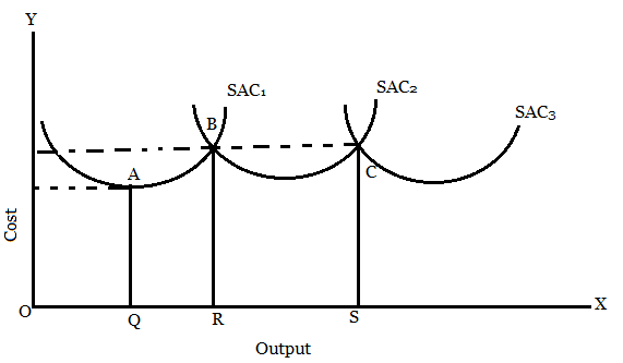 In the above figure, SAC1 refers to the short run average cost curve for the smallest plant, SAC2 is for medium size plant and SAC3 is relation for the large size plant. In the short period, when the output demanded is OQ the firm will choose the smallest size plant.
But for OR output firm will choose medium plant and for output OS the firm will choose large size plant. In the long run, the firm can build a plant whose size leads to the lowest average cost for any given output.
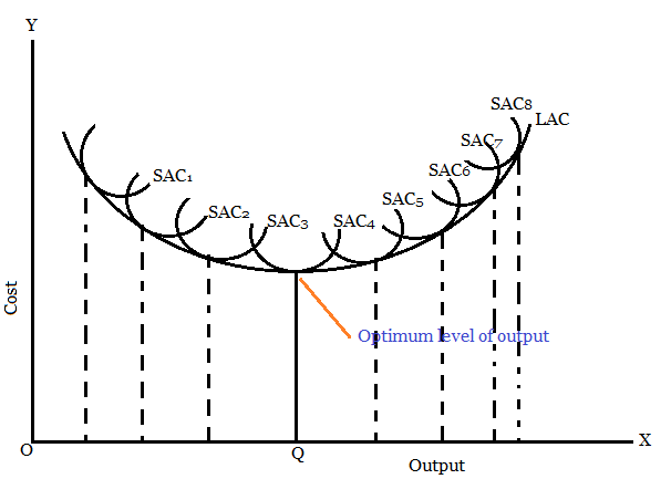
In figure (2), long run average cost curve has been shown the long run average cost curve is tangent to different short run average cost curves. This curve shows the least cost of producing each possible output.
In figure (2), we have drawn a smooth continuous curve connecting the lowest points of a member of SAC curves and have called it as the LAC curve. It is the locus of points representing the least unit cost of producing different output.
 Therefore, the LAC can be defined as the lowest possible average cost of producing any output when the management has adequate time to make all desirable changes and adjustments. The LAC curve is sometimes called the normal cost curve or the planning curve of a firm.
Since factors are indivisible and variable in the long run, the LAC is ‘U’ shaped. The LAC is also known as ‘envelop’ curve. Because it envelops all the SAC curves.
Normally, a firm has some size of plant and a corresponding SAC curve. But over a period of time, the firm can move from one plant size to another. It passes from one SAC curve to another finding a different one at each point on the LAC curve.
The normal relation of the LAC curve to the SAC curve is really a relation of one LAC curve to a family of SAC curves.
FAQs
What is long run average cost curve?
Long run average cost is the long run total cost divided by the total product.
What is the Full form of LAC?
LAC full form in economics is Long run average cost.
What is the full form of SAC?
SAC full form is Short run Average Cost.
Conclusion
So friends, this was the derivation of Long-run average cost curve. Hope you get the full details about it and hope you like this article.
If you like this article, share it with your friends and turn on the website Bell icon, so don’t miss any articles in the near future. Because we are bringing you such helpful articles every day. If you have any doubt about this article, you can comment us. Thank You!
Read More Article
• Relationship between Investment and Rate of Interest
• What is producer equilibrium? | Producer equilibrium class 11